
0 Views
Department of Economics, Vijayanagara Srikrishnadevaraya University, Bellary-583105.
Climate change significantly impacts the consumption patterns of farmers. Crop output and quality are affected, resulting in changes in revenues and profits. Given that the agricultural households are producer -consumers, changes in profits translate as changes in disposable incomes, affecting their consumption. This study analyses the changes in consumption resulting from climatic changes after accounting for socio economic factors using heteroscedasticity consistent least squares estimators. Results indicated that consumption increased with increase in climatic factors such as minimum temperature, water deficit and decreased with increase in maximum temperature, rainfall and wind speeds. However, these changes are not statistically significant across social categories among farmers. Farm size is found to be a significant determinant of consumption.
KEYWORDS: Climate Change, consumption function, Farmer’s consumption, Socio Economic analysis.
Climate change significantly impacts the consumption patterns of farmers. Changes in climate affect the crop production directly. Changes in crop output and quality resulting from climatic changes affect revenues and profits. Agricultural households act as producer -consumers, allocating the profits generated out of the current crop towards investment and consumption. Hence, changes in profits translate into changes in disposable incomes, affecting the consumption. Consumption is an indicator of socio- economic wellbeing of an economic agent. Consumption provides utility to an individual, and hence, increase in consumption expenditure indicated increase in utility obtained by the individual. Consumption includes expenditure on food and non-food items. This study considers family as a unit for analysing consumption. Consumption depends on economic factors such as, disposable income, savings, agronomic factors such as size of the farm, crop revenues; social factors such as education, social status etc. The objectives of this study are to analyse the determinants of consumption and to estimate the impact of climatic change on consumption, after accounting for agronomic, social and economic conditions faced by the agent.
Previous studies analysed various economic and social factors affecting consumption. Murari et al. (2018) found an inverse relation between maximum temperatures and crop yields in rice, sorghum (jowar), finger millet (ragi) and pigeon pea crops in Karnataka at all quantile levels of crop yields. Down to Earth (2019) reported a decline in annual trends in rainfall across Karnataka. However, Sanjeevaiah et al. (2021) found that monotonic increases in rainfall during crop growing season especially June and August months, affected the season onset and yields. Rao et al. (2013) found that an increase of 2°C temperature coupled with 10 per cent decrease in rainfall reduced the yields by 4 per cent. Areef et al. (2021) found that monthly percapita expenditure on consumption and per capita income increased with farm size. Also, share of food items in consumption decreased with farm size. Agronomic factors were also identified as significant in affecting consumption of farmers. Aditya et al. (2019) found that annual and seasonal weather risks significantly influence savings among rural households. Based on these past studies, an attempt is made here to analyse consumption using heteroscedasticity consistent least squares estimators.
Agronomic data used in this study was obtained from ICRISAT’s Village level Dynamics of South Asia (VDSA) SAT II database and Directorate of Economics and Statistics (DES). The data set utilized in the study is a village level panel data from 2009 to 2018, covering 18 villages, 09 districts across the states of Karnataka, Maharashtra, Madhya Pradesh, Gujarat, Andhra Pradesh and Telangana. In each village, 40 households were sampled to represent landless labour, small farmers, medium and large farmers. These households are primarily dependent on farming income. Climate data is combined from Indian Meteorological Department and ICRISAT’s District Level Dataset (DLD), spanning over 120 years, from 1900 to 2020 is used. Data from all these sources is collated and organized into a SAS Database in the year 2021. SAS SQL, SAS IML, and Base SAS routines were utilized for analysis.
Climate data is constructed using weather data on each district. Climate normal for variables such as temperature, rainfall, water deficit and wind speed are calculated as moving average of thirty years. For example, normal temperature for the year 2016 is an average of temperatures recorded for years 1986 through 2015. Similarly, normal temperature for the year 2017 is an average for the years 1987 through 2016. Period of thirty years is used for calculating climate normal from weather data as per the convention in the literature. According to Gerald et al. (2009) the climate change (temperature increase, rainfall decrease, in all season shift) makes agriculture more vulnerable. Average monthly maximum and minimum temperatures were considered in this study.
Temperatures play a significant role in crop growth. An increase in minimum temperatures could extend the growing season and the growing degree days. Crops that require cooler temperatures may find rising minimum temperatures as detrimental. However, most crops may find the increased growing in temperatures to be beneficial. The monthly minimum temperature varied within a range of 5.7 °C (Min 19.96 °C to Max 25.6°C, mean 22.7°C). Coefficient of variation is 7 per cent. The parameter estimate on minimum temperature could be positive.
Average monthly maximum temperature varied within a range of 4.02°C (Min 29.21°C to Max 33.23°C, mean 30.9°C). Coefficient of variation is 3.2 per cent. Increase in maximum temperatures could affect plant growth adversely. Higher temperatures could result in reduction of yields and a reduction in farm revenue. The parameter estimate on maximum temperature is hypothesized to be negative. Quantum and distribution of rainfall is an important factor given the predominance of rainfed farming. Monthly rainfall (month of September) varied within a range of 91 mm (Min 60.64 mm, Max
152.09 mm). Coefficient of variation is 22 per cent. Increase in rainfall could increase the crop yields and revenues, hence the parameter estimate on rainfall is hypothesized to be positive. Monthly average wind speed (month of July) were considered in this study. Wind speed ranged at 1.39 (Min 2.25, Max 3.64). Coefficient of variation of wind speed is 13 per cent. Higher wind speeds can reduce the yields and resultant revenues.
Impacts of temperature, humidity or other microclimatic conditions could be aggravated by increased wind speeds. Saltation of surface soils can physically injure crop plants. Plants can be physically injured, toppled due to higher wind speeds. Parameter estimate on wind speeds is hypothesized to be negative. Water deficit during crop growing season could affect the crop yields negatively. Monthly water deficit (month of August) during the preliminary stages of crop is considered in this study; observed range of water deficit was 61.73 (Min 0, Max 61.73). Coefficient of variation of water deficit is 91.7 per cent parameter estimate on rainfall is hypothesized to be negative.
Demographic variables such as family size, social category of the farming household are also significant determinants of consumption. Large sized families could consume more compared to smaller sized families. Wider distribution of age among family members could influence the consumption patterns, such as expenditure on education or marriage celebrations. Parameter estimate on family is hypothesized to be positive. Social category of the farming household could also influence the consumption. Practices and customs idiosyncratic to the social classes could dictate the patterns in consumption. Different social categories are represented as dummy variables to capture these fixed effects that are specific to the social categories. For example, dummy variable SC takes the value of 1 if the farming household belongs to the scheduled caste category and a value of 0 if the farming household belongs to any other category. 10 per cent of farming households in the data fall under this category. Similarly, variables ST (5% of households), OBC (1% of total households) are defined. The sign on parameters on these variables could not be readily predicted.
Agronomic variables such as size of farm are also important determinants of consumption. Large farmers account for 22 per cent of data, medium farmers account for 23 per cent of data, small farmers account for 32 per cent of data and landless labourers account for 21 per cent of data, respectively. Larger farm size could be associated with higher consumption. This variable is hypothesised to be positive.
Revenue generated from cropping is the main source of income for the farming households. Higher consumption is associated with higher income. Revenue varied within a range of 17.26 lakh Rupees (1.72 million Rs). Coefficient of variation is 166 per cent. Parameter estimate for revenue variable is hypothesised to be positive. Farmer households held their savings predominantly in the form of ornamental gold. The value
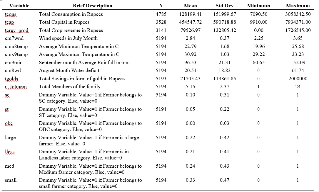
range is 20 lakh Rupees (2 million Rs) with a CV of 167 per cent across the pooled data. Parameter estimate is hypothesised to be positive, given that an increase in long run savings could lead to increases in consumption.
Consumption is the dependent variable in this study. It included expenditure on food and non-food items. Share of food expenditure varies from 21 per cent to 30 per cent across households of different farm sizes. Consumption range was 30.5 Lakh Rupees (3 million Rs), with a CV of 118 per cent.
Y = Xβ + ε Equation 1
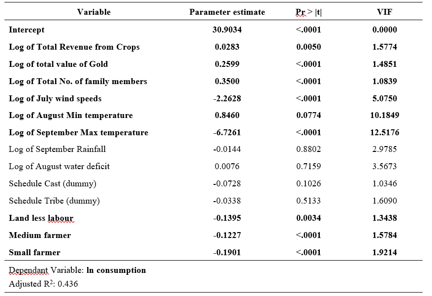
Consumption function has been estimated under Least squares framework as in Equation 1. Consumption is the dependent variable y, and economic, demographic and climatic factors described in the previous section represent the independent variables X, β represents the parameters to be estimated and ϵ is the random error term. Heteroscedasticity Consistent least squares estimation method is utilized in this study. PROC REG procedure of SAS was utilised for estimating the model. Multicollinearity is expected in this model. Variance Inflation Factors (VIFs) were calculated to diagnose the level of multicollinearity. VIF values greater than 10 are an indication of multicollinearity.
Results from the estimated model are presented in Table 2. The estimated VIF values showed that, the model did not suffer from multicollinearity. The model explains about 43 per cent of variability in the dependent variable (Adjusted R2=0.4365). Parameter estimate on crop revenues is positive and significant (0.0283) as hypothesized. An increase in crop revenue leads to an increase in the consumption, after controlling for all other factors. Our results indicate that with a 1 per cent increase in crop revenues, the consumption increases by 0.02 per cent. This parameter could also be interpreted as marginal propensity to consume. The sign on the parameter is in accordance with previous studies. Parameter estimate on savings as indicated by amount of gold owned is positive and significant. A 1 per cent increase in savings leads to an increase of 0.25 per cent in consumption. The savings observed in this model are cumulative over time and in the long run. An increase in long run savings indicates a betterment of economic and social status of an agent. Hence, increases in long run savings is positively correlated with consumption. Parameter estimate on total number of family members is positive and significant, indicating that consumption increases with increase in family members. A 1 per cent increase in family size causes an increase of 0.35 per cent increase in consumption.
Parameter estimates on Climatic variables are predominantly significant and show signs as hypothesized. Wind speeds are negatively associated with consumption. A 1 per cent increase in wind speed results in a 2.26 per cent decrease in consumption. Higher wind speeds can cause a reduction in crop revenues, as wind can exacerbate water losses, prevailing heat conditions, rainfall and can also cause physical damage to the plant. Parameter estimate on Average minimum temperatures is positive and significant. A 1 per cent increase in minimum temperature leads to an increase in consumption by 0.84 per cent. Increase in minimum temperatures could mean additional growing degree days resulting in higher revenues. Parameter estimate on average maximum temperature is negative and statistically significant. The results indicate that a 1 per cent increase in maximum temperature results in a decrease of consumption by 6.72 per cent. Higher maximum temperatures could reduce the performance of the crop plants, reducing the resulting crop revenues. Parameter estimates on rainfall and water deficit variables are not statistically significant.
Parameter estimates on farm size are statistically significant. Small farmers experienced more reduction in consumption compared to Land less agricultural labour and medium famers. Parameter estimates on Demographic variables such as social category of the farmer were not statistically significant. However, the farmers belonging to the SC category and ST category experienced more reduction in consumption compared to other categories of farmers. SC category famers experienced more reduction in consumption compared to the ST category farmers. These differences were not statistically significant.
Climate change significantly impacts the consumption patterns of farmers. This study analysed the changes in consumption of agricultural households as a function of climatic variables after controlling for economic, agronomic and demographic factors. Our results indicate that with a 1 per cent increase in crop revenues, the consumption increases by 0.02 per cent. Crop revenues are the main source of income for agricultural households. Changes in income affect the consumption directly. Higher consumption is associated with higher incomes. Agricultural households held their savings predominantly in the form of gold (ornamental). Higher value in gold savings is an indicator of economic betterment and is associated with social status. Results
from our model indicate that higher the long run savings in gold, higher is the consumption associated. Besides the economic factors, family size and farm size are also statistically significant determinants of consumption. Higher the levels of family size and farm size, higher is the associated consumption of the household.
Climatic variables affect the household consumption significantly. Increase in average maximum temperatures has more pronounced impacts than comparative increase in minimum temperature. The results indicate that a 1 per cent increase in maximum temperature results in a decrease of consumption by 6.72 per cent, whereas a 1 per cent increase in minimum temperature leads to an increase in consumption by 0.84 per cent. Wind speeds also affect consumption. A 1 per cent increase in wind speeds results in a 2.26 per cent decrease in consumption. Changes in rainfall, and water deficit during the growing season were not found to be statistically significant in the estimated model. Results from this model could be of use to policy makers in designing better suited relief packages that mitigate weather related or climate related
disasters.
Authors would like to thank ICSSR IMPRESS funding this project under Grant No.P1686/142. Also, Authors express their gratitude to ICRISAT for providing access to their Databases.
Aditya, R.K., Ashok, K.M and Nedumaran, S. 2019. Consumption, habit formation, and savings: Evidence from a rural household panel survey. Review of Development Economics. 23(1):1-19.
Areef, M., Radha, Y., Rao, V.S., Gopal, P.V.S., Paul, K.S.R., Suseela, K and Rajeswari, S. 2021. Consumption expenditure pattern and inequality among agricultural households in south coastal region of Andhra Pradesh State. Journal of Research ANGRAU. 49(2): 82-91.
Down to Earth. 2019. Rainfall trends decline sharply across regions in Karnataka. Retrieved from website (https://www.downtoearth.org.in/news/ climate-change/rainfall-trends-decline-sharply- across-regions-in-karnataka-64893) on 27.09.2021.
Gerald, C.N., Mark, W.R., Jawoo, K., Richard, R., Timothy, S., Tingju, Z., Claudia, R., Siwa, M., Amanda, P., Miroslav, B., Marilia, M., Rowena, V.S., Mandy, E and David, L. 2009. Climate change: Impact on agriculture and costs of adaptation. International Food Policy Research Institute (IFPRI) Washington, D.C. USA.
Murari, Kamal, K., Mahato, Sandeep, Jayaraman, T and Swaminathan, M. 2018. Extreme temperatures and crop yields in Karnataka, India. Review of Agrarian Studies. 8(2).
Rao, A.V.R.K., Wani, S.P., Srinivas, K., Singh, P., Bairagi, S.D and Ramadevi, O. 2013. Assessing impacts of projected climate on pigeon pea crop at Gulbarga. Journal of Agrometeorology. 15 (Special Issue-II): 32-37.
Sanjeevaiah, S.H., Rudrappa, K.S., Lakshminarasappa, M.T., Huggi, L., Hanumanthaiah, M.M., Venkatappa, S.D., Lingegowda, N and Sreeman,
S.M. 2021. Understanding the temporal variability of rainfall for estimating agro-climatic onset of cropping season over south interior Karnataka, India. Agronomy. 11(6):1135.